Linear Regression (Math)

Linear Regression (Math)

Linear regression is a fundamental statistical and machine learning technique used to model the relationship between a dependent variable (denoted as Y) and one or more independent variables (denoted as X). It assumes a linear relationship between these variables.

Simple Linear Regression

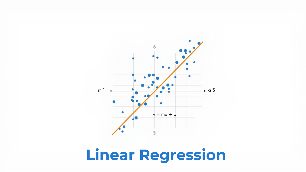
Simple linear regression is a statistical method used to model the relationship between a dependent variable and a single independent variable. The relationship is modeled as a linear equation.

Equation:

y = c + mx

Where:

• y: Dependent variable (output, response, or predicted variable). This is the variable we are trying to predict.
• x: Independent variable (input, predictor, or explanatory variable). This is the variable we use to make predictions.
• m: Slope of the line (regression coefficient). It represents the change in y for every one-unit change in x.
• c: Intercept (constant). It represents the value of y when x is zero. This is the point where the regression line crosses the y-axis.

Goal:

The primary goal of simple linear regression is to find the "best fit" line by determining the optimal values for m (slope) and c (intercept). These values minimize the difference between the predicted values of y (based on the linear equation) and the actual observed values of y in the data. This optimization is often achieved using the method of least squares.

Multiple Linear Regression

Multiple linear regression is a statistical technique that extends simple linear regression to model the relationship between a dependent variable (also known as the response variable or outcome variable) and two or more independent variables (also known as predictor variables or explanatory variables). Unlike simple linear regression, which uses only one independent variable, multiple linear regression allows for a more complex and potentially more accurate representation of the factors influencing the dependent variable.

Core Concept:

The goal of multiple linear regression is to find the best linear equation to predict the value of the dependent variable based on the values of the independent variables. This equation takes the form:

Y = β₀ + β₁X₁ + β₂X₂ + ... + βₙXₙ + ε

Where:

• Y is the dependent variable.
• X₁, X₂, ..., Xₙ are the independent variables.
• β₀ is the y-intercept (the value of Y when all X variables are zero).
• β₁, β₂, ..., βₙ are the coefficients (also known as slopes or regression weights) for each independent variable. They represent the change in Y for a one-unit change in the corresponding X variable, holding all other X variables constant. This "holding all others constant" is a crucial aspect of interpreting coefficients in multiple regression.
• ε is the error term (also known as the residual), representing the difference between the actual value of Y and the value predicted by the model. It accounts for the variability in Y that is not explained by the independent variables.

Key Assumptions:

Multiple linear regression relies on several key assumptions to ensure the validity of the results:

• Linearity: The relationship between the independent variables and the dependent variable is linear. This means that a straight-line relationship can adequately describe the association. This can be visually checked using scatter plots of each independent variable against the dependent variable, or a plot of residuals versus predicted values.

• Independence: The errors (residuals) are independent of each other. This means that the error for one observation should not be correlated with the error for another observation. This is particularly important when dealing with time series data. This is often assessed using the Durbin-Watson test for autocorrelation. A Durbin-Watson statistic close to 2 suggests no autocorrelation.

• Homoscedasticity: The variance of the errors is constant across all levels of the independent variables. This means the spread of the residuals should be roughly the same for all predicted values. This is checked using a scatter plot of residuals vs. predicted values. A funnel shape in the plot suggests heteroscedasticity (non-constant variance).

• Normality: The errors are normally distributed. This assumption is most critical for hypothesis testing and confidence interval estimation. This can be checked using a histogram or Q-Q plot of the residuals. The Q-Q plot should show the residuals falling approximately along a straight line if they are normally distributed.

• No Multicollinearity: The independent variables are not highly correlated with each other. High multicollinearity can lead to unstable coefficient estimates and difficulty in interpreting the individual effects of the predictors. Variance Inflation Factor (VIF) is a common measure of multicollinearity. VIF values above 5 or 10 are often considered indicative of problematic multicollinearity.

Advantages of Multiple Linear Regression:

• Improved Prediction: Can often provide more accurate predictions than simple linear regression by incorporating multiple relevant factors.
• Understanding Relationships: Helps to understand the individual and combined effects of multiple independent variables on a dependent variable.
• Control for Confounding Variables: Allows for controlling the effects of confounding variables, providing a more accurate estimate of the relationship between the variables of interest.

Disadvantages of Multiple Linear Regression:

• Complexity: Can be more complex to interpret and implement than simple linear regression.
• Data Requirements: Requires sufficient data to accurately estimate the model parameters, especially as the number of independent variables increases. A common rule of thumb is to have at least 10-20 observations for each independent variable.
• Sensitivity to Assumptions: Violation of the assumptions can lead to biased or unreliable results.
• Overfitting: With a large number of independent variables, there's a risk of overfitting the model to the training data, resulting in poor performance on new data. Techniques like regularization (e.g., Ridge, Lasso) and cross-validation can help mitigate overfitting.

Applications:

Multiple linear regression is widely used in various fields, including:

• Economics: Modeling economic growth, predicting consumer spending.
• Finance: Predicting stock prices, assessing investment risk.
• Marketing: Analyzing the effectiveness of advertising campaigns, predicting customer behavior.
• Healthcare: Identifying risk factors for diseases, predicting patient outcomes.
• Social Sciences: Studying factors influencing educational attainment, analyzing social trends.

Example:

Suppose you want to predict a house's price (Y) based on its size in square feet (X₁), number of bedrooms (X₂), and location (represented by a numerical score X₃). A multiple linear regression model could be used to estimate the coefficients β₀, β₁, β₂, and β₃ to build the prediction equation:

House Price = β₀ + β₁(Size) + β₂(Bedrooms) + β₃(Location Score) + ε

The coefficients would then tell you how much the house price is expected to change for each additional square foot, bedroom, or point on the location score, holding the other variables constant. For instance, β₁ represents the expected change in house price for a one-square-foot increase in size, assuming the number of bedrooms and location score remain the same.